Reconstitution & Titration
Peptide Dose Lab
Nothing is pre-set for you.
Vial & syringe inputs
Enter what's on your vial label and how much you're drawing up.
Insulin syringes are marked in "units" based on a standard where 1 mL = 100 units, regardless of the syringe's physical capacity — a 0.3 mL syringe just has fewer unit lines. Double-check your reading against the syringe in hand before drawing anything.
Weekly dose & weight loss log
Log what you actually took each week — the chart below builds itself from this table.
Weekly dose chart
Bars show dose per week; the line (if you logged weight) tracks body weight on its own axis.
Log
| Wk | Date | Dose | Weight | Notes |
|---|
Save / load your data
Everything lives in this browser tab only — export a JSON file to keep it, and load it back in anytime (here or on another device).
How to add dosing protocols to Google calendar
Pro Tips
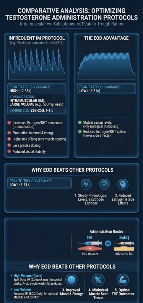
Frequency beats total dose — EOD or 3x weekly gives smoother levels and less aromatization than once-weekly, even at the same total dose.
Match frequency to ester length — Short esters need EOD or daily. Medium esters work best 2–3x weekly.
Split long-ester doses — 80 mg + 80 mg+ 80 mg 3 times weekly is often better than 250 mg once weekly. Many men cut their AI dose by 50% or more.
AI timing is critical — Never take AI on injection day. Wait 12–24 hours after the peak (usually 12–24 h post-shot).
Rotate injection sites — Glute, quad, delt, or subQ. Rotate to avoid scar tissue and pain.
Split peptides — Most peptides (BPC, TB-500, Ipamorelin, CJC, GHRP) work best split into 2–3 daily doses.
Find your personal sweet spot — After 2–3 cycles, use the frequency that gives smooth energy, good libido, and trough bloodwork closest to your target range.
Oral steroids — Take them daily or as a short kick (front-loaded weeks 1–4). Cycle length is usually shorter than injectables. Can also be used a backloaded cycle towards the last weeks.
Track everything — Add simple notes per plan (site, time, AI taken, how you felt). You’ll see what actually works for your body.
Cycle Calculator
Plot blood-level curves for anabolic compounds, TRT & peptides using pharmacokinetic modelling
This plotter uses a first-order single-compartment elimination model. Each injection adds a dose bolus, which then decays exponentially according to the compound's elimination half-life. Accumulation from repeated dosing is handled by summing all active boluses at each time point.
Where available, elimination half-life t½, time to peak Tmax, and bioavailability are drawn from peer-reviewed human studies. For compounds with limited published data, estimates are derived from structural analogy to related esters or preclinical models.
| Compound | t½ | Tmax | Ester / Form | Source / Reference |
|---|
| Compound | t½ | Tmax | Notes | Source / Reference |
|---|
| Compound | t½ | Tmax | Notes | Source / Reference |
|---|
| Compound | t½ | Tmax | Notes | Source / Reference |
|---|
What is the Y-axis?
The Y-axis shows relative blood-level concentration in arbitrary units proportional to your entered dose (mg or mcg). It is not an absolute serum testosterone value in ng/dL or nmol/L — actual blood levels depend on individual metabolism, injection site, body composition, and many other factors.
Think of the Y-axis as a shape indicator: it accurately shows you when levels peak, trough, and reach steady-state, even if the exact number doesn't match a lab result.
What is the X-axis?
The X-axis is time in weeks from the start of your cycle. Week 0 is injection day 1. The chart extends 2 weeks past your selected cycle length so you can see the washout/clearance tail. Gridlines mark each week.
What does the curve shape mean?
- Rising phase (weeks 1–4 typically): Each injection adds more compound than has been cleared. Blood levels climb toward steady-state.
- Plateau / steady-state: The amount injected per interval equals the amount eliminated. The curve flattens into a saw-tooth wave — peaks right after each injection, troughs just before the next.
- Clearance tail (after last injection): No new compound is added; levels fall exponentially. The steeper the fall, the shorter the half-life.
Key pharmacokinetic terms explained
- Half-life (t½)
- The time it takes for blood concentration to fall to 50% of its current level. A compound with a 5-day half-life loses half its concentration every 5 days. Longer half-life = slower rise to steady-state, slower clearance.
- Tmax
- Time to peak concentration after a single injection. Testosterone Enanthate has a Tmax of ~2 days — so levels peak roughly 2 days after each shot, then decline.
- Steady-state
- Achieved after approximately 4–5 half-lives of continuous dosing. For Test E (t½ ~4.5 days), this is roughly 3–4 weeks. At steady-state, average levels stabilise between your trough and peak values.
- Accumulation
- With frequent dosing or long half-lives, each dose adds on top of residual levels from previous doses. This is why weekly Test E injections build up over several weeks rather than reaching full levels on day 1.
- Trough
- The lowest point in blood level, occurring just before your next injection. This is typically when side effects from low levels (low mood, libido) are felt, and when most bloodwork is done to measure stable trough levels.
- Peak
- The highest point after an injection. Occurs at Tmax. Large peak-to-trough swings (common with long esters dosed infrequently) can cause side effects at both ends.
- AUC
- Area Under the Curve — the total exposure over time, found by integrating concentration over the plotted window. Two protocols can share the same peak but have very different AUC if one holds levels high for longer.
- Peak/trough ratio
- Peak concentration divided by trough concentration during a steady-state dosing interval. A ratio close to 1 means very stable levels (frequent small doses); a high ratio means big swings (infrequent large doses).
Reading the metric cards
- Peak value: The maximum concentration your model predicts at any point in the cycle.
- Avg (steady-state): The average level during the middle 30% of your cycle — a rough estimate of your steady-state concentration.
- AUC: Total area under that compound's curve across the whole plotted window — a single number for "total exposure."
- Peak/trough ratio: How much levels swing within one dosing interval once at steady-state.
Using the controls
- From / Through week: Lets you model kickstarters (short oral compounds in weeks 1–4), or compounds that are dropped mid-cycle. Each compound runs only between these weeks.
- Offset (days): Delays the first injection by this many days. Useful if you want Compound B to start mid-week relative to Compound A, or to model a front-load timing offset.
- Level adjustment slider (±100%): Scales a compound's output up or down. Use it to model lower absorption (−20%), compare conservative vs. aggressive dosing, or represent bioavailability differences between individuals.
- Schedule: Injection frequency. More frequent injections (e.g. every other day for short esters) flatten peak-to-trough swings and are generally considered more stable. Less frequent injections create larger swings.
- Custom compound: Pick "+ Custom compound…" at the bottom of the compound dropdown to enter your own name, half-life (in hours or days), and dose unit. It plugs straight into the same PK model as the built-in compounds.
Saving, comparing & exporting
- Save current protocol: Stores everything you've entered (compounds, doses, schedules, dates) in this browser's local storage, under the protocol name you gave it.
- Overlay: Draws a saved protocol's combined curve as a dashed line on top of whatever you're currently editing, so you can compare two approaches at a glance.
- Export / Import JSON: Download all saved protocols as a single .json file (for backup, or to move them to another browser/device), or load a previously exported file back in.
- PNG export: Saves exactly what's drawn on the chart — including any overlays — as an image file.
- Email: Builds a plain-text summary (compounds, doses, schedules, and the metrics above) and opens it in your default email app as a draft. Nothing is sent without you doing so yourself.
- Add to Google Calendar: Opens a recurring event per compound, starting from your protocol's start date and repeating on its dosing schedule until the "through week." Fractional schedules (like 3× per week) are rounded to the nearest whole-day interval, since calendar recurrence rules need integer days.
- Download calendar file (.ics): Same events as above, bundled into one file you can import into Google Calendar, Outlook, Apple Calendar, or hand off to someone else (e.g. a training partner or coach).
Why doesn't my chart match my bloodwork?
This calculator uses published population-average pharmacokinetic values. Your actual levels depend on:
- Individual metabolism (faster or slower clearance)
- Injection depth and site (IM vs. subQ, glute vs. delt)
- Oil vehicle and concentration of the compound
- Body composition (body fat affects ester storage/release)
- The assay used by your lab (LC-MS/MS vs. immunoassay)
Use the Level adjustment slider to calibrate the model against your own bloodwork results. If your trough bloodwork reads ~20% lower than the chart shows, dial that compound to −20%.